40 how to format data labels in excel charts
Formatting Long Labels in Excel - PolicyViz Copy your graph Open PowerPoint and Paste the graph. Don't worry about the slide size or anything, just paste it in. Select the axis you want to format and select the Format option in the Paragraph menu. In the ensuing menu, select the Right option in the Alignment drop-down menu. How to Create and Customize a Waterfall Chart in Microsoft ... Double-click the chart to open the Format Chart Area sidebar. Then, use the Fill & Line, Effects, and Size & Properties tabs to do things like add a border, apply a shadow, or scale the chart. Select the chart and use the buttons on the right (Excel on Windows) to adjust Chart Elements like labels and the legend, or Chart Styles to pick a theme ...
How to Create and Customize a Treemap Chart in Microsoft Excel Either right-click the chart and pick "Format Chart Area" or double-click the chart to open the sidebar. On Windows, you'll see two handy buttons on the right of your chart when you select it. With these, you can add, remove, and reposition Chart Elements. And you can pick a style or color scheme with the Chart Styles button.

How to format data labels in excel charts
Prevent Overlapping Data Labels in Excel Charts - Peltier Tech Apply Data Labels to Charts on Active Sheet, and Correct Overlaps Can be called using Alt+F8 ApplySlopeChartDataLabelsToChart (cht As Chart) Apply Data Labels to Chart cht Called by other code, e.g., ApplySlopeChartDataLabelsToActiveChart FixTheseLabels (cht As Chart, iPoint As Long, LabelPosition As XlDataLabelPosition) Improve your X Y Scatter Chart with custom data labels Press with right mouse button on on a chart dot and press with left mouse button on on "Add Data Labels" Press with right mouse button on on any dot again and press with left mouse button on "Format Data Labels" A new window appears to the right, deselect X and Y Value. Enable "Value from cells" Select cell range D3:D11 Formatting Charts in Excel - GeeksforGeeks You can add Data Labels by using the "+" button on the top right corner of the chart. Now open the Format Data Labels Window and can change the Font color, size, alignment, and many other options. 4. Formatting Data Series: You can change the color of the bar charts by selecting them and then open the "Format Data Series" window.
How to format data labels in excel charts. support.microsoft.com › en-us › officeFormat a Map Chart - support.microsoft.com You should see the Format Object Task Pane on the right-hand side of the Excel window. If the Series Options aren't already displayed, then click the Series Option expander button on the right side and select the Series "value" option that corresponds with your data. Next, select the Series Options button to display the Series Options and Color ... How to: Display and Format Data Labels | .NET File Format ... To apply a number format to data labels, utilize the DataLabelBase.NumberFormat property, which provides access to the NumberFormatOptions object containing format options for displaying numbers in different chart elements. Next, assign the corresponding number format code to the NumberFormatOptions.FormatCode property. datacycleanalytics.com › how-to-create-advanced4 steps: How to Create Waterfall Charts in Excel 2013 - Data ... May 13, 2016 · Add data labels by right-clicking one of the series and selecting “Add data labels…” Add labels to each of the series apart from the invisible column. Select the data labels and make them bold, change colour as appropriate. The finished chart should look something similar to the one below. Download the completed version here. How To Add Axis Labels In Excel [Step-By-Step Tutorial] Axis labels make Excel charts easier to understand.. Microsoft Excel, a powerful spreadsheet software, allows you to store data, make calculations on it, and create stunning graphs and charts out of your data.. And on those charts where axes are used, the only chart elements that are present, by default, include:
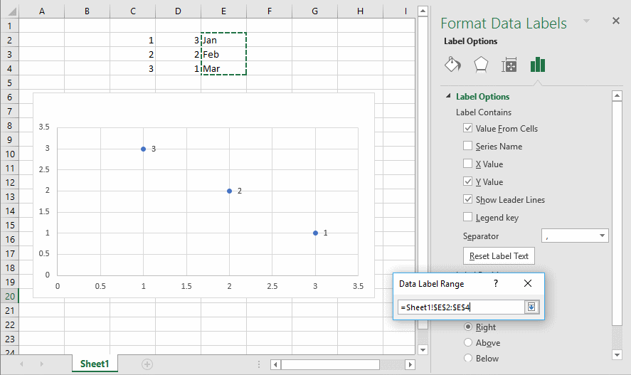
Excel Pivot Table Filter and Label Formatting - Microsoft ... Excel 2016. Images of 2 separate workbooks, each with a data table, pivot table and pivot chart, the one on the right created by copy & paste of the one on the left. The one on the right changed: X axis labels on the pivot chart don't have the multi-level option. Also, unlike the original on the left, there is now a filter button for the chart. How to Find, Highlight, and Label a Data Point in Excel ... By default, the data labels are the y-coordinates. Step 3: Right-click on any of the data labels. A drop-down appears. Click on the Format Data Labels… option. Step 4: Format Data Labels dialogue box appears. Under the Label Options, check the box Value from Cells . Step 5: Data Label Range dialogue-box appears. Custom Chart Data Labels In Excel With Formulas Follow the steps below to create the custom data labels. Select the chart label you want to change. In the formula-bar hit = (equals), select the cell reference containing your chart label's data. In this case, the first label is in cell E2. Finally, repeat for all your chart laebls. DataLabels object (Excel) | Microsoft Docs With Charts(1).SeriesCollection(1) .HasDataLabels = True .DataLabels.NumberFormat = "##.##" End With Use DataLabels (index), where index is the data-label index number, to return a single DataLabel object. The following example sets the number format for the fifth data label in series one in embedded chart one on worksheet one.
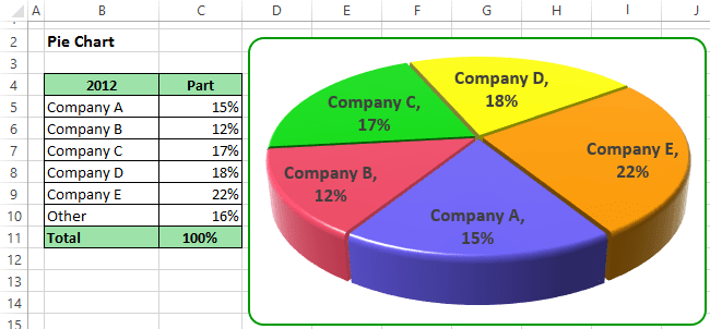
Slope Chart with Data Labels - Peltier Tech It can be done manually, but Excel first adds default labels above the points showing just the values. We need to select the labels for each series individually to add the series names, then we need to select the left and right labels separately to position them to the left of the left category or to the right of the right category. Bo-o-o-oring! excel - Formatting Data Labels on a Chart - Stack Overflow sub charttest () activesheet.chartobjects ("chart 6").activate z = 1 with activechart if .charttype = xlline then i = .seriescollection (1).points.count activechart.fullseriescollection (1).datalabels.select for pts = 1 to i activechart.fullseriescollection (1).points (pts).hasdatalabel = true ' make sure all points are visible data … Change the format of data labels in a chart Data labels make a chart easier to understand because they show details about a data series or its individual data points. For example, in the pie chart below, without the data labels it would be difficult to tell that coffee was 38% of total sales. You can format the labels to show specific labels elements like, the percentages, series name, or category name. Excel: How to Create a Bubble Chart with Labels - Statology Then click OK and in the Format Data Labels panel on the right side of the screen, uncheck the box next to Y Value and choose Center as Label Position. The following labels will automatically be added to the bubble chart: Step 4: Customize the Bubble Chart. Lastly, feel free to click on individual elements of the chart to add a title, add axis ...
Excel 2016 charts: How to use the new Pareto, Histogram, and Waterfall formats | PCWorld
Exactly how to Make a Bar Chart in Microsoft Excel ... When your information is selected, click Insert > > Insert Column or Bar Chart. Various column charts are offered, yet to insert a typical bar graph, click the "Clustered Chart" alternative. This graph is the very first symbol noted under the "2-D Column" section. Excel will automatically take the data from your data set to produce the ...

Do My Excel Blog: How to design a multiple clustered bar chart series in Excel
How to color chart bars based on their values (Chart data is made up) This article demonstrates two ways to color chart bars and chart columns based on their values. Excel has a built-in feature that allows you to color negative bars differently than positive values. You can even pick colors. You need to use a workaround if you want to color chart bars differently based on a condition.

Elements of an Excel Chart | ExcelDemy.com
Chart.ApplyDataLabels method (Excel) | Microsoft Docs For the Chart and Series objects, True if the series has leader lines. Pass a Boolean value to enable or disable the series name for the data label. Pass a Boolean value to enable or disable the category name for the data label. Pass a Boolean value to enable or disable the value for the data label.

Microsoft Excel Tutorials: The Chart Layout Panels
Bar Chart in Excel - Types, Insertion, Formatting - Excel ... To insert a bar chart from this data:-. Select the source data A1:B13. Go to the Insert tab on the ribbon. Click on the Recommended Charts button, this opens the Insert Chart dialog box. Navigate to the All Charts tab and choose the Clustered Bar Chart. Click Ok. This inserts the bar chart as shown in the preview.

Do My Excel Blog: How to design a multiple clustered bar chart series in Excel
Format Chart Axis in Excel - Axis Options (Format Axis ... However, In this blog, we will be working with Axis options, Tick marks, Labels, Number > Axis options> Axis options> Format Axis Pane. Axis Options: Axis Options There are multiple options So we will perform one by one. Changing Maximum and Minimum Bounds The first option is to adjust the maximum and minimum bounds for the axis.

How to Add Data Labels in Excel - Excelchat | Excelchat
How to Add Labels to Scatterplot Points in Excel - Statology Step 3: Add Labels to Points Next, click anywhere on the chart until a green plus (+) sign appears in the top right corner. Then click Data Labels, then click More Options… In the Format Data Labels window that appears on the right of the screen, uncheck the box next to Y Value and check the box next to Value From Cells.

34 Label Chart In Excel - Labels Database 2020
Text Labels on a Horizontal Bar Chart in Excel - Peltier Tech Dec 21, 2010 · In this tutorial I’ll show how to use a combination bar-column chart, in which the bars show the survey results and the columns provide the text labels for the horizontal axis. The steps are essentially the same in Excel 2007 and in Excel 2003. I’ll show the charts from Excel 2007, and the different dialogs for both where applicable.

Excel Charts | Real Statistics Using Excel
How to Create a Run Chart in Excel (2021 Guide) | 2 Free ... Download this Excel run chart template with dynamic data labels. Note: Since your median is going to be different, you need to adapt the custom number formatting accordingly ( Format Data Labels > Label Options > Number > Format Code > In the " Format Code " field, replace " 80 " with your median value as shown below).
Excel 3-D Pie charts - Microsoft Excel 2013
› charts › dynamic-chart-dataCreate Dynamic Chart Data Labels with Slicers - Excel Campus Feb 10, 2016 · Step 3: Use the TEXT Function to Format the Labels. Typically a chart will display data labels based on the underlying source data for the chart. In Excel 2013 a new feature called “Value from Cells” was introduced. This feature allows us to specify the a range that we want to use for the labels.

Microsoft Excel Tutorials: The Chart Layout Panels
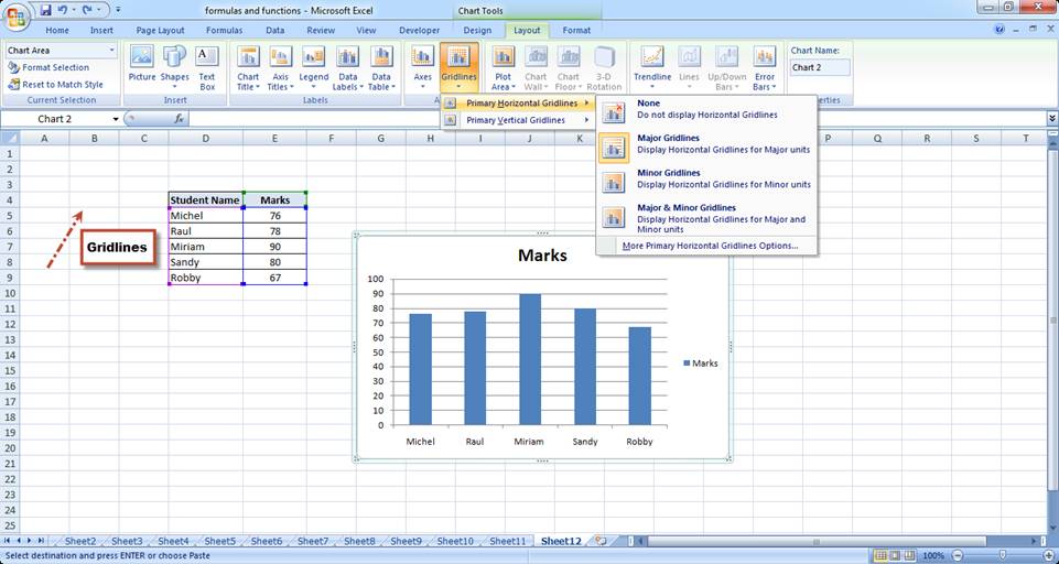
Creating and Modifying Charts - Using Microsoft Excel ... In all cases, you have to select the chart first to access Chart Tools. To add any labels (for example, the title or axes), under the Design ribbon, click Add Chart Element in the Chart Layouts group and select the desired label. To change the chart type, data, or location, use the Chart Tools Design ribbon.
Add Labels to Chart Data in Excel - YouTube
excel - Adding Data Label To Chart Based On X Values ... Categories, including maybe "Red" in column A, Values in column B, and chart labels in column C. In cell C2 I'm using a formula like this: =IF (A2="Red","Label Text Here","") so there is only text in that column if the X value is "Red". My chart plots columns A and B of the data range.
Moving X-axis labels at the bottom of the chart below negative values in Excel - PakAccountants.com
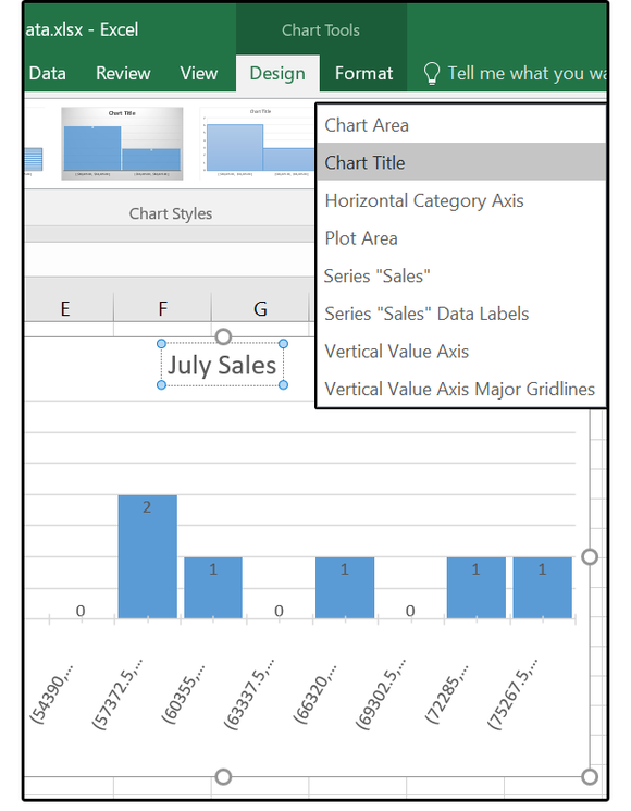
Format Data Labels in Excel- Instructions - TeachUcomp, Inc. 14/11/2019 · To format data labels in Excel, choose the set of data labels to format. To do this, click the “Format” tab within the “Chart Tools” contextual tab in the Ribbon. Then select the data labels to format from the “Chart Elements” drop-down in the “Current Selection” button group. Then click the “Format Selection” button that appears below the drop-down menu in the same …

How to Add Data Labels to your Excel Chart in Excel 2013 - YouTube
Pivot Chart Data Label Formatting Question - Microsoft ... I format the data labels, for example make the text larger or turn it. Every time I refresh the data the data label formatting reverts to the default. I have gone to the Pivot Chart options and made sure the Preserve cell formatting option is checked. How to I get around this and preserve my data label formatting when the data is refreshed?
Custom data labels in a chart
Best Types of Charts in Excel for Data Analysis ... 29/04/2022 · #4 Use a clustered column chart when the data series you want to compare are of comparable sizes. So if the values of one data series dwarf the values of the other data series, then do not use the column chart. For example, in the chart below, the values of the data series ‘Website Traffic’ completely dwarf the values of the data series named ‘Transactions’:

Format Number Options for Chart Data Labels in Excel 2011 for Mac
data-flair.training › blogs › types-of-charts-in-excelTypes of Charts in Excel - DataFlair 11. Stock Charts in Excel. The user uses the stock charts to view the fluctuations in the stock prices. These charts are also useful to view the fluctuations in other datasets such as daily temperature, rainfall, etc. To make use of the stock charts, the data should be in a specific order. This chart compares the aggregate values of several ...
Basic Excel Chart Formatting - MS Excel Charting Tutorial Part 4 | Vertical Horizons
How to format bar charts in Excel — storytelling with data Click on any data label to highlight them all, then right-click and choose Format Data Labels: 4. In the Format Data Labels menu, select Label Options, and in the Label Positions section, choose Inside End. (While you're at it, in the Label Contains section, uncheck "Show Leader Lines." These are almost never necessary.)

Excel Dashboard Templates How-to Use Data Labels from a Range in an Excel Chart - Excel ...
How to Print Labels from Excel - Lifewire Choose Start Mail Merge > Labels . Choose the brand in the Label Vendors box and then choose the product number, which is listed on the label package. You can also select New Label if you want to enter custom label dimensions. Click OK when you are ready to proceed. Connect the Worksheet to the Labels
Post a Comment for "40 how to format data labels in excel charts"