43 how to change category labels in excel chart
Edit titles or data labels in a chart - support.microsoft.com Edit the contents of a title or data label that is linked to data on the worksheet In the worksheet, click the cell that contains the title or data label text that you want to change. Edit the existing contents, or type the new text or value, and then press ENTER. The changes you made automatically appear on the chart. Top of Page How to use cell values for excel chart labels - How to Select the chart, choose the "Chart Elements" option, click the "Data Labels" arrow, and then "More Options." Uncheck the "Value" box and check the "Value From Cells" box. Select cells C2:C6 to use for the data label range and then click the "OK" button. The values from these cells are now used for the chart data labels ...
Custom Data Labels with Colors and Symbols in Excel Charts - [How To ... Step 3: Turn data labels on if they are not already by going to Chart elements option in design tab under chart tools. Step 4: Click on data labels and it will select the whole series. Don't click again as we need to apply settings on the whole series and not just one data label. Step 4: Go to Label options > Number.
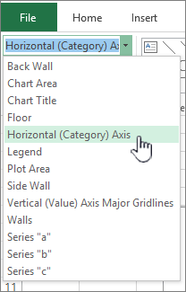
How to change category labels in excel chart
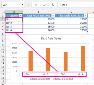
Change axis labels in a chart - support.microsoft.com Right-click the category labels you want to change, and click Select Data. In the Horizontal (Category) Axis Labels box, click Edit. In the Axis label range box, enter the labels you want to use, separated by commas. For example, type Quarter 1,Quarter 2,Quarter 3,Quarter 4. Change the format of text and numbers in labels How to Change Bar Chart Color Based on Category in Excel (3 ... - ExcelDemy Steps: First, select the ranges B4:B11 and D4:D11. After that, go to Insert >> Bar Chart >> 2D Bar Chart. Next, you will see the bars in the Bar Chart of the Profit value in the same color. The negative profit value or the loss amounts are situated on the left side of the chart. How to Add Two Data Labels in Excel Chart (with Easy Steps) For instance, you can show the number of units as well as categories in the data label. To do so, Select the data labels. Then right-click your mouse to bring the menu. Format Data Labels side-bar will appear. You will see many options available there. Check Category Name. Your chart will look like this.
How to change category labels in excel chart. How do I format the second level of multi-level category labels 1. Are the chart inserted in chart sheet? If so, move it to regular sheet and check if it helps. 2. How did you create labels in the chart from the scratch? Please provide the steps to reproduce and verify the results. 3. How exactly you wish the labels to be aligned? Reply with necessary information and I'll be happy to assist you further. How To Add Data Labels In Excel - luanhong.us To do this, click the format tab within the chart tools contextual tab in the ribbon. Use the following steps to add data labels to series in a chart: Source: pakaccountants.com. Add custom data labels from the column x axis labels. In this second method, we will add the x and y axis labels in excel by chart element button. Add or remove data labels in a chart - support.microsoft.com Click Label Options and under Label Contains, pick the options you want. Use cell values as data labels You can use cell values as data labels for your chart. Right-click the data series or data label to display more data for, and then click Format Data Labels. Click Label Options and under Label Contains, select the Values From Cells checkbox. How to Customize Your Excel Pivot Chart Data Labels - dummies If you want to label data markers with a category name, select the Category Name check box. To label the data markers with the underlying value, select the Value check box. In Excel 2007 and Excel 2010, the Data Labels command appears on the Layout tab. Also, the More Data Labels Options command displays a dialog box rather than a pane.
How to Edit Pie Chart in Excel (All Possible Modifications) How to Edit Pie Chart in Excel 1. Change Chart Color 2. Change Background Color 3. Change Font of Pie Chart 4. Change Chart Border 5. Resize Pie Chart 6. Change Chart Title Position 7. Change Data Labels Position 8. Show Percentage on Data Labels 9. Change Pie Chart's Legend Position 10. Edit Pie Chart Using Switch Row/Column Button 11. Excel Chart Data Labels-Modifying Orientation - Microsoft Community Answer. You can right click on the data label part then select Format Axis. Click on the Size & Properties tab then adjust the Text Direction or Custom Angle. Was this reply helpful? How to Add Category Labels AND Data labels to the Same Bar Chart in ... #excel #dataviz #barchartHere's a great trick for when you need your bar chart's category label appear on one side of the bar and your data label to appear o... Data Labels in Excel Pivot Chart (Detailed Analysis) Next open Format Data Labels by pressing the More options in the Data Labels. Then on the side panel, click on the Value From Cells. Next, in the dialog box, Select D5:D11, and click OK. Right after clicking OK, you will notice that there are percentage signs showing on top of the columns. 4. Changing Appearance of Pivot Chart Labels
Individually Formatted Category Axis Labels - Peltier Tech Format the category axis (vertical axis) to have no labels. Add data labels to the secondary series (the dummy series). Use the Inside Base and Category Names options. Format the value axis (horizontal axis) so its minimum is locked in at zero. You may have to shrink the plot area to widen the margin where the labels appear. Change the format of data labels in a chart To get there, after adding your data labels, select the data label to format, and then click Chart Elements > Data Labels > More Options. To go to the appropriate area, click one of the four icons ( Fill & Line, Effects, Size & Properties ( Layout & Properties in Outlook or Word), or Label Options) shown here. How to Change Axis Labels in Excel (3 Easy Methods) Firstly, right-click the category label and click Select Data > Click Edit from the Horizontal (Category) Axis Labels icon. Then, assign a new Axis label range and click OK. Now, press OK on the dialogue box. Finally, you will get your axis label changed. That is how we can change vertical and horizontal axis labels by changing the source. Change axis labels in a chart in Office - support.microsoft.com Change the text of category labels in the source data Use new text for category labels in the chart and leavesource data text unchanged Change the format of text in category axis labels Change the format of numbers on the value axis Related information Add or remove titles in a chart Add data labels to a chart Available chart types in Office
Change the display of chart axes
How to Add Two Data Labels in Excel Chart (with Easy Steps) For instance, you can show the number of units as well as categories in the data label. To do so, Select the data labels. Then right-click your mouse to bring the menu. Format Data Labels side-bar will appear. You will see many options available there. Check Category Name. Your chart will look like this.

Changing Axis Labels in PowerPoint 2013 for Windows
How to Change Bar Chart Color Based on Category in Excel (3 ... - ExcelDemy Steps: First, select the ranges B4:B11 and D4:D11. After that, go to Insert >> Bar Chart >> 2D Bar Chart. Next, you will see the bars in the Bar Chart of the Profit value in the same color. The negative profit value or the loss amounts are situated on the left side of the chart.
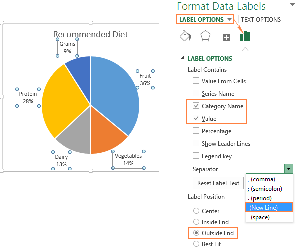
How to make a pie chart in Excel
Change axis labels in a chart - support.microsoft.com Right-click the category labels you want to change, and click Select Data. In the Horizontal (Category) Axis Labels box, click Edit. In the Axis label range box, enter the labels you want to use, separated by commas. For example, type Quarter 1,Quarter 2,Quarter 3,Quarter 4. Change the format of text and numbers in labels
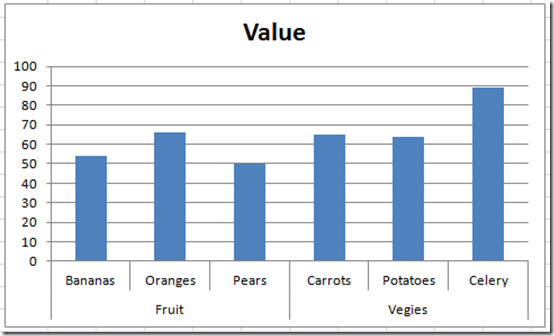
Fixing Your Excel Chart When the Multi-Level Category Label ...
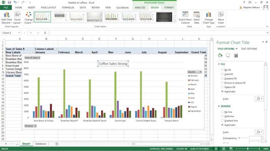
How to Customize Your Excel Pivot Chart and Axis Titles - dummies
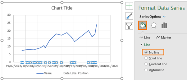
Label Specific Excel Chart Axis Dates • My Online Training Hub
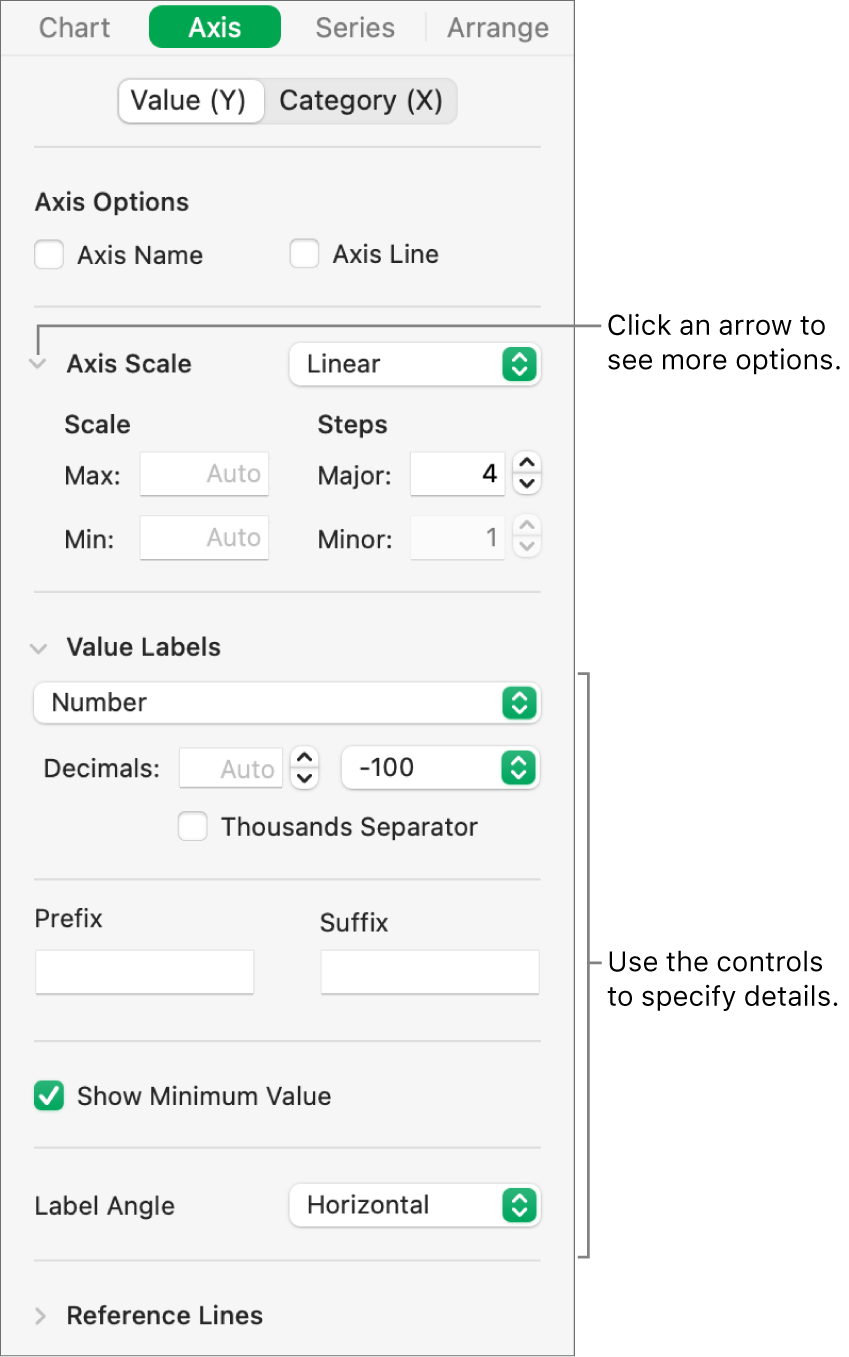
Change the look of chart text and labels in Numbers on Mac ...

Format Data Labels in Excel- Instructions - TeachUcomp, Inc.

Add horizontal axis labels - VBA Excel - Stack Overflow
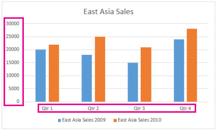
Change axis labels in a chart
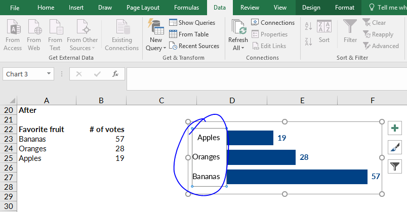
How to Sort Your Bar Charts | Depict Data Studio

Adding rich data labels to charts in Excel 2013 | Microsoft ...
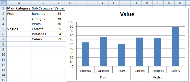
Fixing Your Excel Chart When the Multi-Level Category Label ...
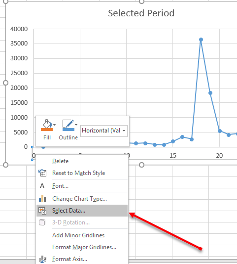
Change Horizontal Axis Values in Excel 2016 - AbsentData
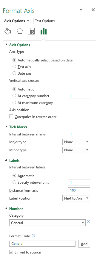
Change the display of chart axes
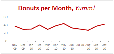
Show Months & Years in Charts without Cluttering » Chandoo ...
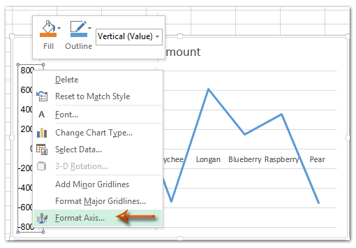
How to change chart axis labels' font color and size in Excel?
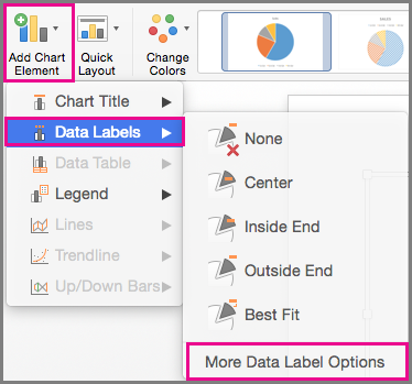
Change the format of data labels in a chart

Bar charts with long category labels; Issue #428 November 27 ...
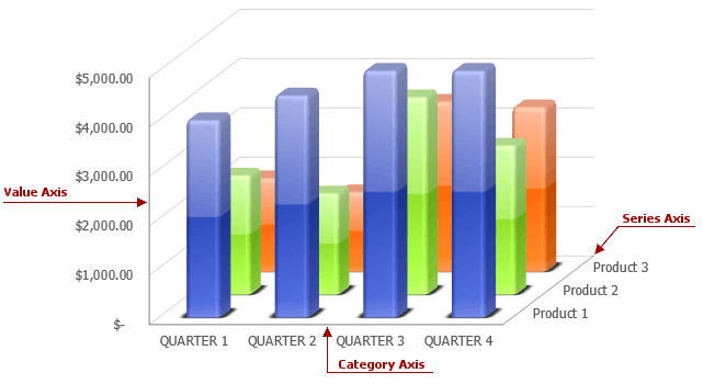
How to: Change the Display of Chart Axes | .NET File Format ...
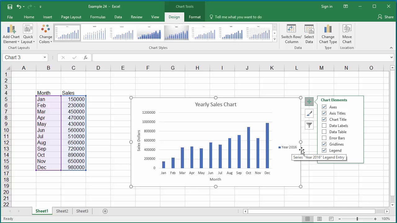
How to Change Elements of a Chart like Title, Axis Titles, Legend etc in Excel 2016
3 Ways to Make Excel Chart Horizontal Categories Fit Better ...

Add Labels ON Your Bars
Change axis labels in a chart
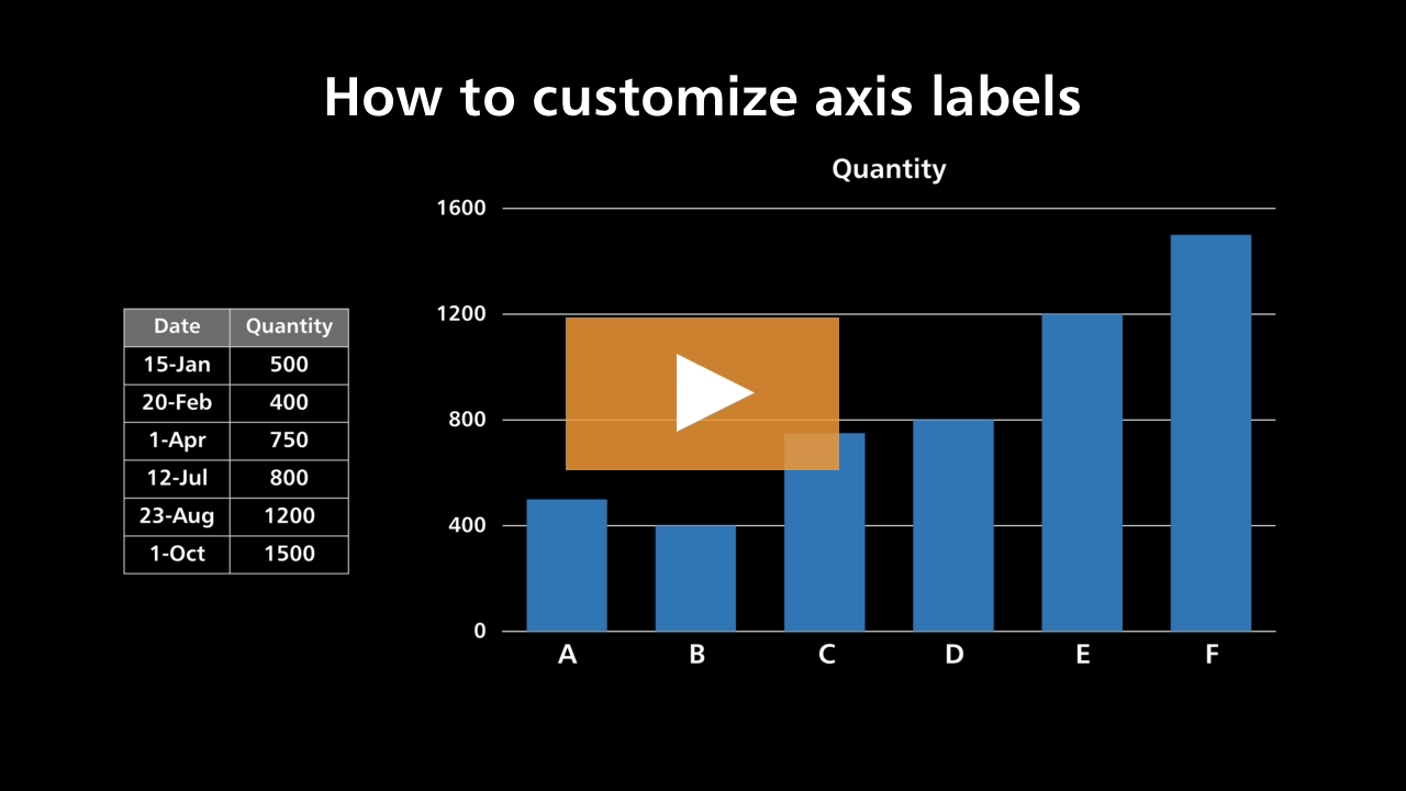
How to customize axis labels
How to change a line chart axis scale in Office 365 Excel - Quora
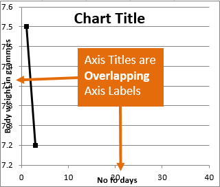
Resize the Plot Area in Excel Chart - Titles and Labels Overlap
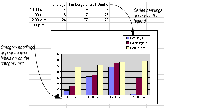
Working With Chart Data Ranges
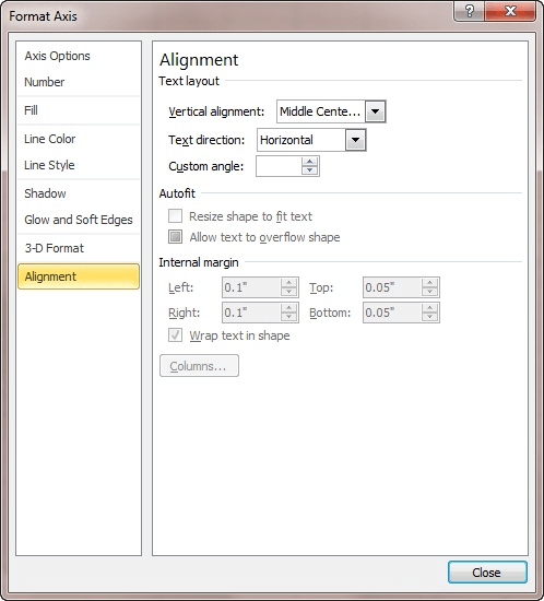
Adjusting the Angle of Axis Labels (Microsoft Excel)
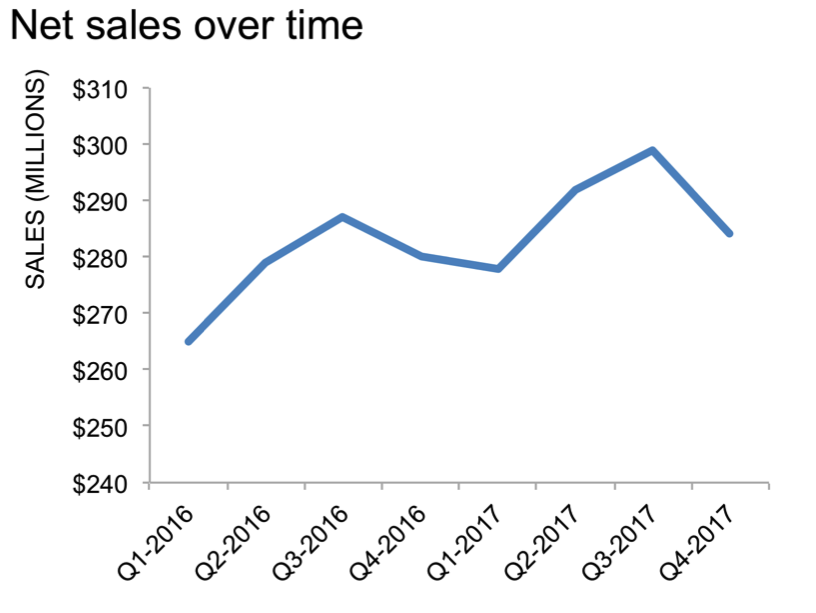
Excel axis labels - supercategory — storytelling with data
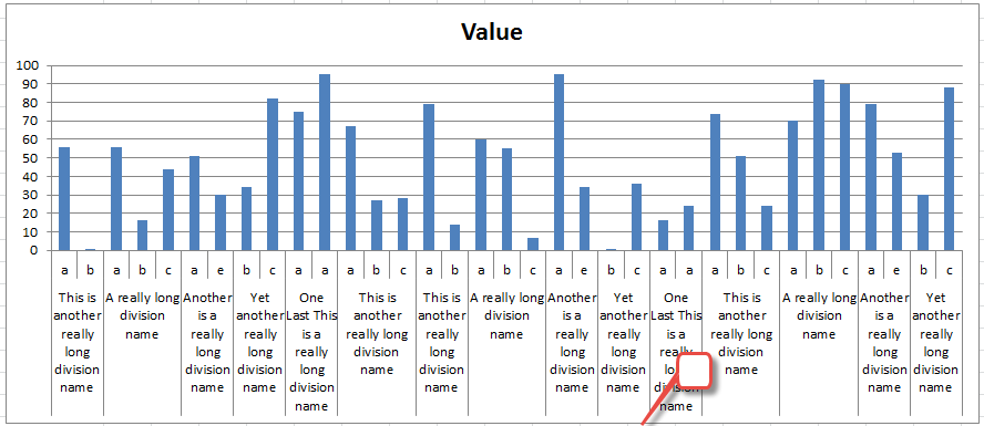
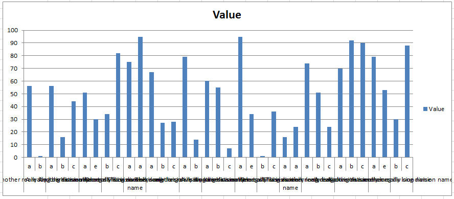
3 Ways to Make Excel Chart Horizontal Categories Fit Better ...
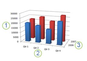
Change the display of chart axes
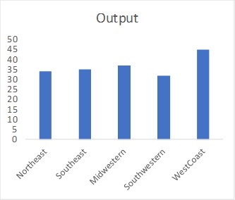
Stagger long axis labels and make one label stand out in an ...
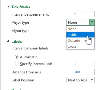
Change the display of chart axes
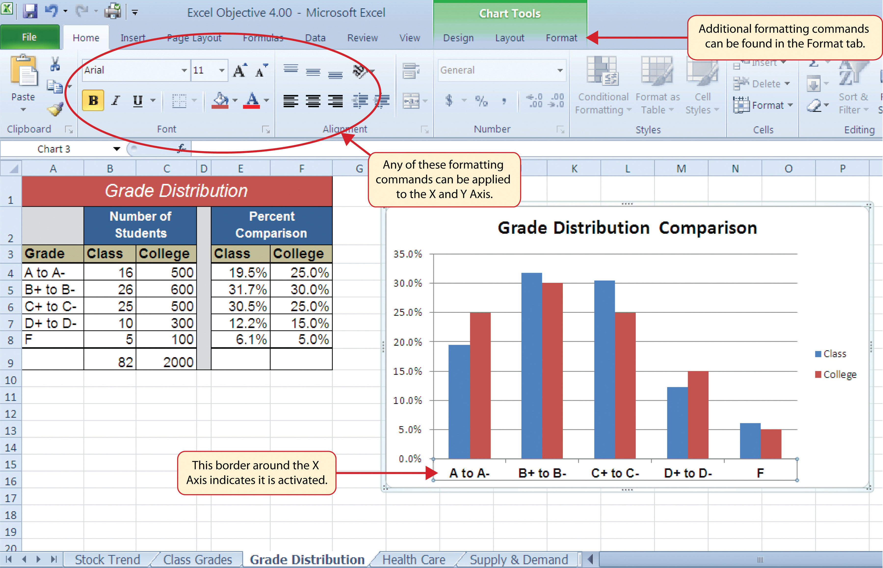
Formatting Charts
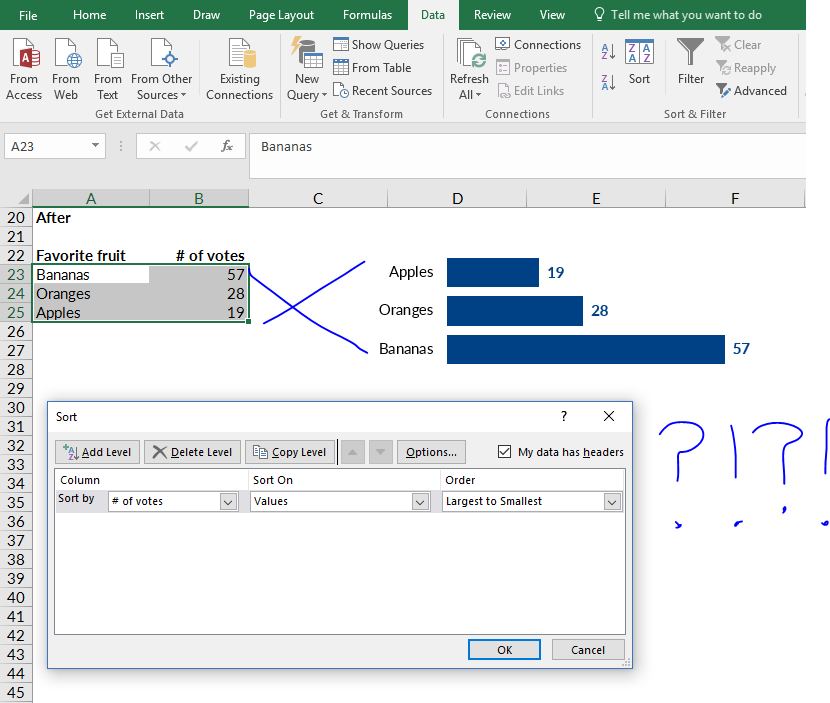
How to Sort Your Bar Charts | Depict Data Studio
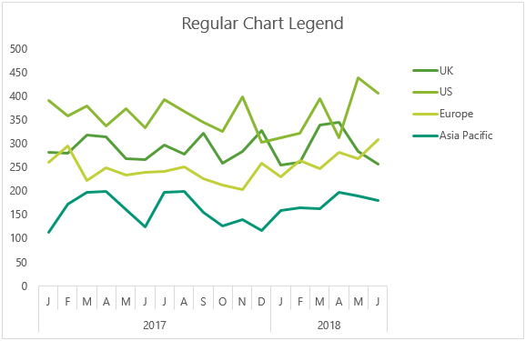
Dynamically Label Excel Chart Series Lines • My Online ...
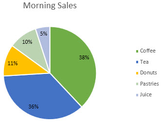
Change the format of data labels in a chart

How to Change Horizontal Axis Labels in Excel | How to Create Custom X Axis Labels
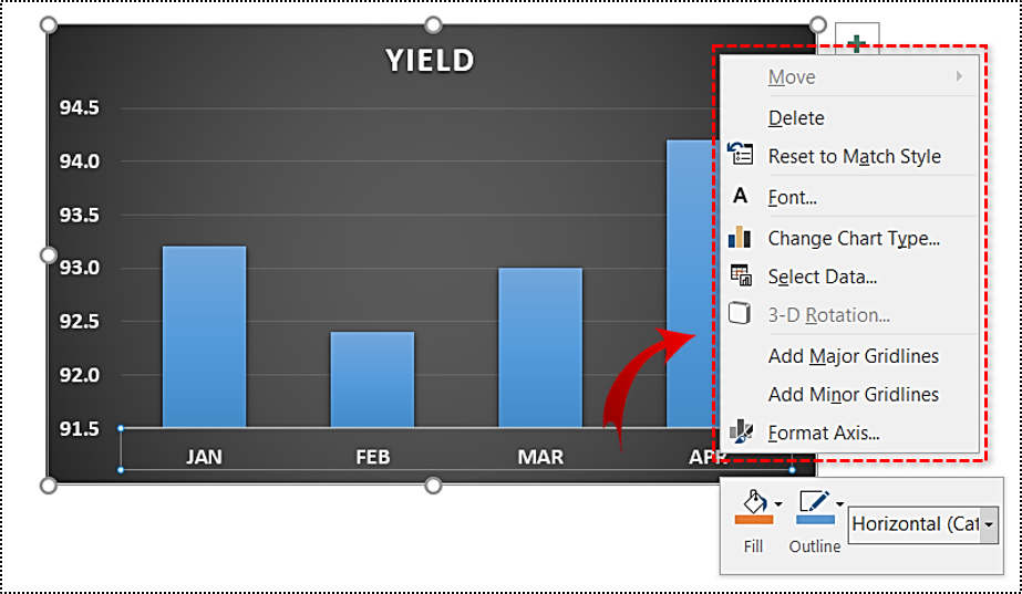
How to Change the X-Axis in Excel

Changing the order of items in a chart

How to Make Excel Pie Chart Examples Videos ◔
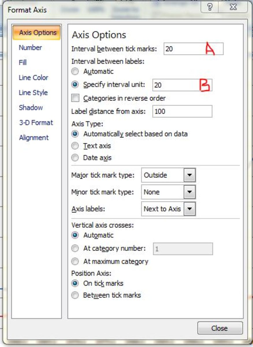
How to Graph and Label Time Series Data in Excel - TurboFuture
Post a Comment for "43 how to change category labels in excel chart"